
library(tidyverse)
library(tidytext)
library(gutenbergr)
library(wordcloud)
library(topicmodels)

# tidy some texts - not used here
# devtools::source_gist("gist.github.com/jmclawson/0773f1200ee4ec47cf25f0a2acecaa26")

# unnest without caps
devtools::source_gist("gist.github.com/jmclawson/79e6994d491b3572d3a31e1f6a29ffc2")

# build and visualize topic models
devtools::source_gist("gist.github.com/jmclawson/640042f2d679bcef1d20cf8056a66acd")1 Introibo
Way back in 2016, I shared some code to standardized a topic-modeling workflow. For one who was still relatively new to R, this workflow helped me speed through the process of creating topic models to the juicy parts of actually reading and understanding what they might show. But when a new computer butted heads with Mallet, I sided with the shiny new hardware and stepped away from topic models.
I got a chance to revisit them this past spring semester when teaching a course in literary text mining. A mixture of students working for their English degree or their certificate in Data Analytics, the class worked through approaches for text mining using Julia Silge and David Robinson’s Tidy Text Mining and Matthew Jockers and Rosamond Thalken’s Text Analysis with R. Because students came to the course with different backgrounds, it was necessary to write some functions to simplify both modelling and visualizing.
These functions had to be documented, so I might as well share them here. (I’ll also continue using them myself, even after the class is done, and I don’t want to forget how!) This blog post, like the documents prepared for class, is written in Quarto, an evolved form of RMarkdown that makes it easy to intersperse text and code, set apart in fenced “code chunks.”
2 Loading up code
First up are the packages and code used. Some functions—including those for creating and visualizing topic models—are defined outside of this Quarto document to keep things tidy.
Links to three source files on GitHub:
- tidy_some_texts.R - to bring in text files that aren’t from Project Gutenberg
- unnest_without_caps.R - for a simple process of removing things that look like proper nouns in English
- topic_model.R - for creating a topic model and visualizing the model a few different ways
3 Getting books
Topic modeling can take a long time, so the examples here will show a small number of books, about the same number students used in their projects.
Before getting too far along, it’s necessary to point out the eval: false flag at the top of certain code chunks. When working inside the document, it’s possible to run this code by itself (for instance, by clicking the green “Run” triangle at the top right of each code chunk in RStudio), but the eval: false flag will keep a chunk from running when a document is rendered. Here, I use the flag to avoid hitting Project Gutenberg’s web servers too many times, simultaneously saving the data locally with saveRDS(). A later chunk will load this file with readRDS().
```{r}
#| label: get-books
#| eval: false
#| message: false
gothic_fiction <-
  gutenberg_download(c(345, 84, 696, 2852, 174), meta_fields = c("title", "author"))

# save the data locally so books only need to bedownloaded once
saveRDS(gothic_fiction, "data/gothic_fiction.rds")
```
4 Doing the work
The process of creating topic models is pretty involved, but it’s also kind of formulaic. The provided function simplifies it all to one step to save confusion. Behind the scenes, the make_topic_model() function completes five steps:
- Removes words I don’t want. Some of these are stop words like “the” and “of” and “and.” Others include words that appear only in a first-letter-capitalized form. This is a quick and sneaky way of dropping proper nouns, since characters’ names can really sabotage a topic model.
- Unnests the table so that it has one word per row. This is a pretty standard step.
- Divides each book into 1,000-word chunks.1 This step allows us to treat each chunk as a similarly-sized document we can measure, thereby understanding how a book’s topics change from its first page to its last.
- Counts the word frequencies and then converts the table into a “document term matrix.” This sounds more complex than it really is. Think of it as converting a table that has one word per row into a table that has one document per row. Each column of this document term matrix represents one of the words being considered, with cells showing the number of times that word was used in each of the documents.
- Builds a topic model, assaying every 1,000-word chunk in every book. If we can understand “topics” as collections of words that appear with each other in similar contexts—compare, for instance, a list of words like “ocean, sea, boat, whale, harpoon, ship” against another list of words like “corn, tractor, field, harvest, rain, soil”—then this step endeavors to sort words into these clumps of ideas. When we set
k=15we tell it to divide all the words up into 15 topics, just ask=30would tell it to find 30 topics.
Step 5 takes a lot of time, so I’ve once again set eval: false at the top of the code chunk so that it won’t get repeated when I render the document. Instead, as before, saveRDS() will save the topic model locally when I run the chunk manually.
```{r}
#| label: make-and-save
#| message: false
#| eval: false

# load up the RDS saved in the previous code chunk
gothic_fiction <- readRDS("data/gothic_fiction.rds") |> select(title, text)

# now build the topic models. "LDA" in these names refers to the topic-model process, so I like to add it to the names to remind me that these aren't tables of data. I'm creating a couple here so that I can test to see if there's a stable point where the number of topics seems to work well. Higher values of k add lots of time!

# limit randomization
set.seed(2222)

# make the model
gothic_lda_10 <- make_topic_model(gothic_fiction, k = 10)

# limit randomization
set.seed(2222)

# make the model
gothic_lda_30 <- make_topic_model(gothic_fiction, k = 30)

# Save the progress so far
saveRDS(gothic_lda_10, "data/gothic_lda_10.rds")
saveRDS(gothic_lda_30, "data/gothic_lda_30.rds")
```
Note
Be aware that topic models rely on randomization, with topics divided up by lots of coin flips. Even with the same set of books and the same number of topics, two topic models are bound to look differently every time you make them. Here, I’m limiting randomization by using the set.seed() function so that results are stable enough to look into. It’s not a bad idea to limit randomization similarly, but only after first comparing a few randomized models to make sure results look more or less similar, and you’re not relying on a fluke.
Now that the RDS files are saved, I can load them back up with a code chunk that doesn’t have eval: false at the top:
gothic_lda_10 <- readRDS("data/gothic_lda_10.rds")
gothic_lda_30 <- readRDS("data/gothic_lda_30.rds")
5 Making pictures
5.1 Visualize document topics
Topic models can be tough to visualize, so these four functions will help. First is visualize_document_topics(), which rejoins each book from its 1,000-word chunks to show a distribution of its most common topics from the beginning to end. It sets some reasonable defaults, but arguments in the function will modify things:
- By default, it will save a .png image in the “plots” folder in the file pane so that images can be used elsewhere. By adding
saveas = "pdf"the file type can be changed to a .pdf file. - Only the four most common topics will be shown per book, but adding
top_n = 5(or some other number) lets you choose how many topics to show. - Other options allow further tweaking:
omit = c(3, 17)to skip plotting some irrelevant topicssmooth = FALSEto increase spikiness (and potentially noise)direct_label = FALSEto use a color legend instead of numbers printed on the graphtitle = FALSEto omit the model name from the chart title.
Here’s my 10-topic model of Gothic fiction, showing a few of these different options in play: a few different
visualize_document_topics(gothic_lda_10,
                          smooth = FALSE,
                          top_n = 4)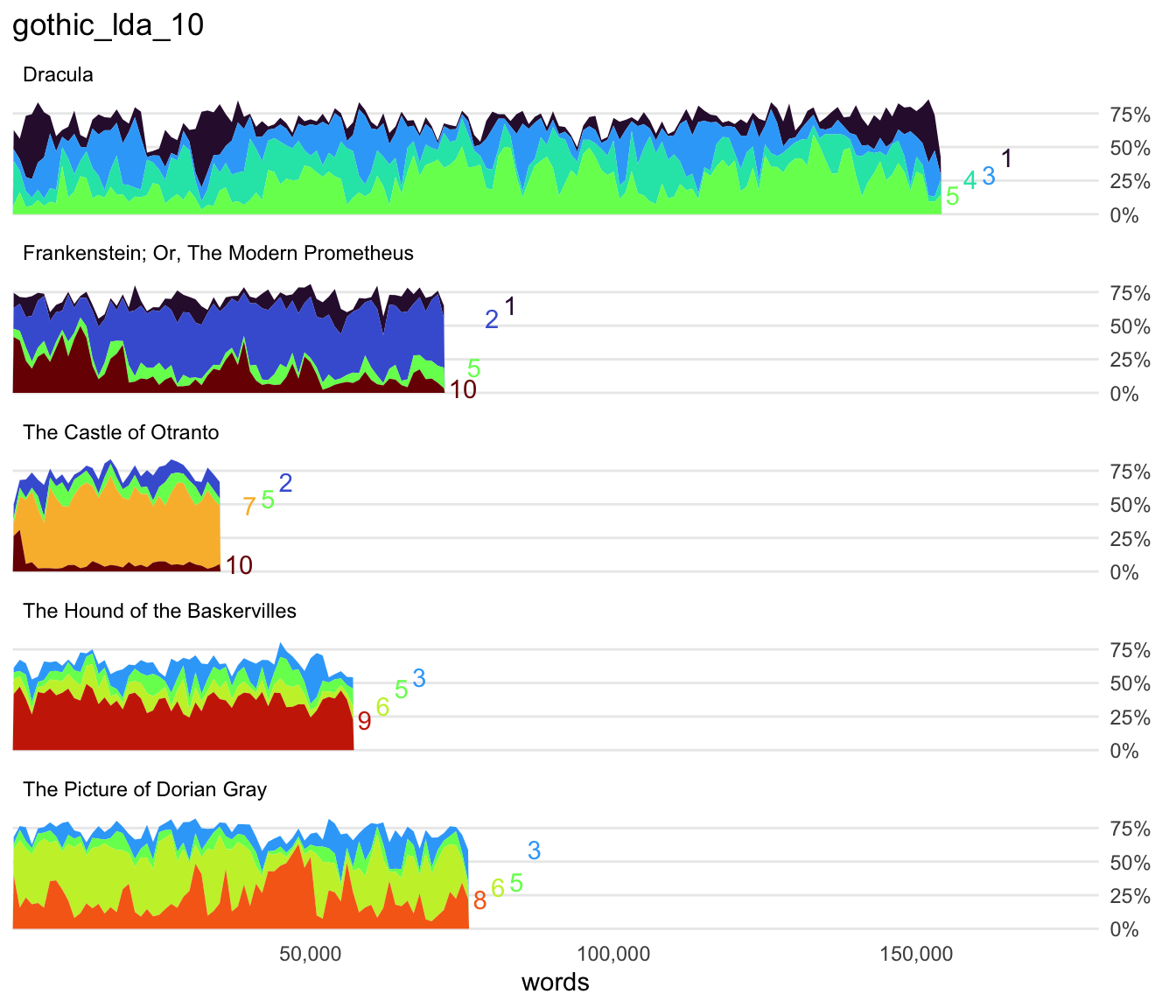
visualize_document_topics(gothic_lda_10,
                          smooth = FALSE,
                          direct_label = FALSE)
visualize_document_topics(gothic_lda_10, saveas = "pdf")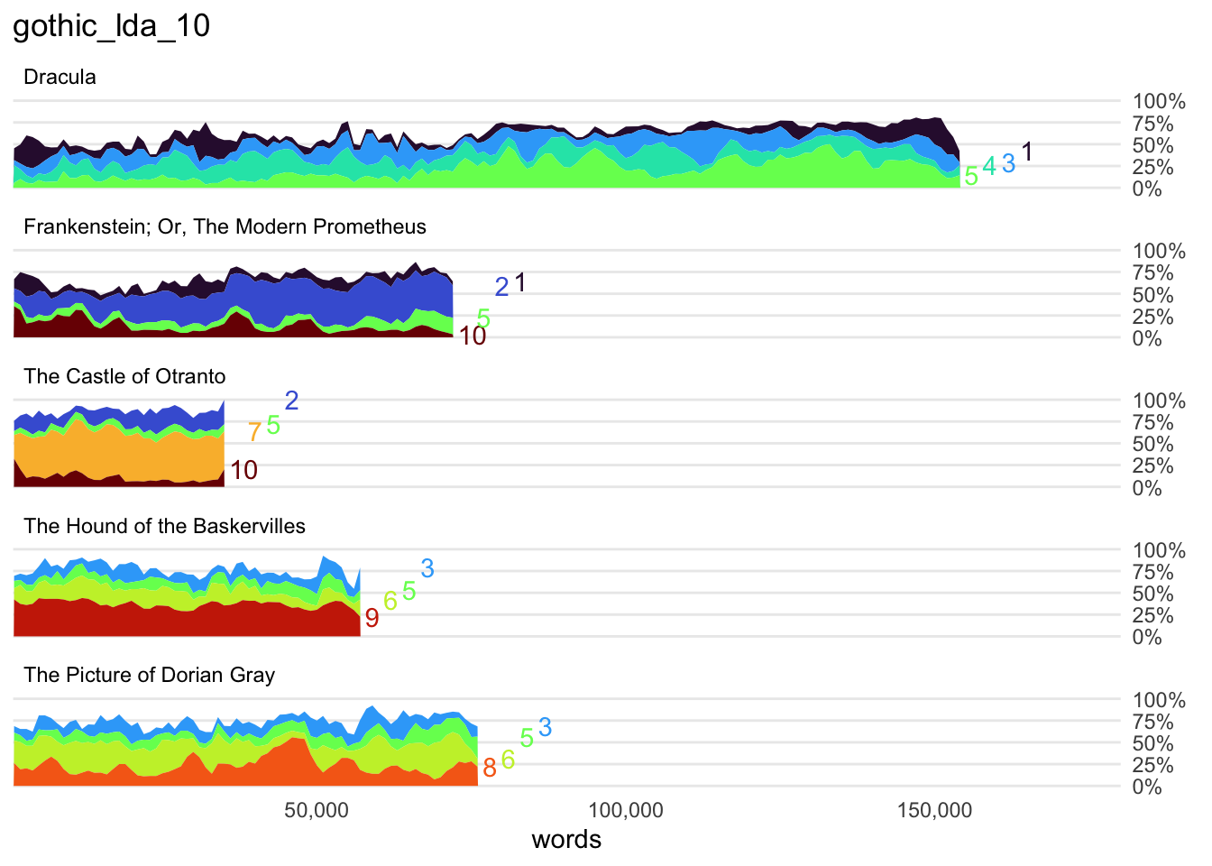
saveas argument makes it easy to export different file types.Notice that the middle one is much spikier, and it uses a legend to distinguish among topics. The first and last look the same, but the latter creates .pdf files of the visualization, which is probably the best looking. You can see the .pdf in the “plots” folder.
While exploring these texts, I actually made a handful of topic models with different numbers of topics—more models than shown here. Results were mixed. In some, topics were very revealing and made sense to me, but others were kind of “junk” piles of miscellaneous words. The model comprising 30 topics was the most satisfying I found for these 5 books, but it’s worth experimenting with different numbers.
Here’s the topic distribution for the model with 30 topics:
visualize_document_topics(gothic_lda_30, saveas = "pdf")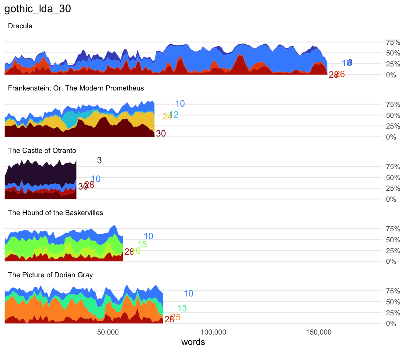
One thing I see here is that some topics like topic 10 are among the top 4 topics in nearly every book. That suggests that it may be a topic related to normal narrative forms like “said” or “says”, or it might be a junk topic of miscellaneous words. Another thing is that The Castle of Otranto has an enormous distribution of topic 3. Since I know that book, I can guess that this is related to archaisms that threw off my topic model. (Darn it!) But I’m intrigued at certain points by some topics that emerge to play an important part of the narrative before fading away. Frankenstein shows a notable swelling of topic 12 halfway through the book. I’m also curious about topic 8 in Dracula, which peeks over the mountaintops a few times. I wonder what these topics can tell me?
To see if there are other important topics that are just out of sight, I’ll expand my visualization from 4 to show the top 6 topics. Keep in mind that adding topics will yield diminishing returns, as each added topic will be less prevalent than the last.
visualize_document_topics(gothic_lda_30, top_n = 6)
top_n parameter will change how many topics are shown.Immediately, my eyes are drawn to topic 21 in Dracula. I’m also curious about topic 17, which pops up briefly in The Picture of Dorian Gray and the momentary showing of topic 5 in Frankenstein. For the purposes of understanding storyline, I’m basically most interested in those topics that jump in to say hello for a chunk of the text but which are otherwise not really seen. But we might also use these approaches to categorize the texts by commonalities. For instance, what does topic 24 suggest is shared between Frankenstein and The Castle of Otranto?
Altogether, I’m curious to explore these topics to see what they tell me about those texts: 12, 8, 21, 17, 5. I’m also curious to see whether topic 10 is significant or junk. Luckily, we have ways to look closer.
5.2 Topics as bars
The function called visualize_topic_bars() will show behind the curtain to see what each “topic” entails. This function prepares a visualization showing the words that play the biggest part in each topic. By default, it shows the top 10 words, but setting top_n = 15 (or some other number) will let you choose how many words to show. Like the previous function, it also saves a copy of this chart in the “plots” folder.
Here’s the function in action, exploring the topics I listed above:
visualize_topic_bars(gothic_lda_30,
                     topics = c(12, 8, 21, 17, 5, 10))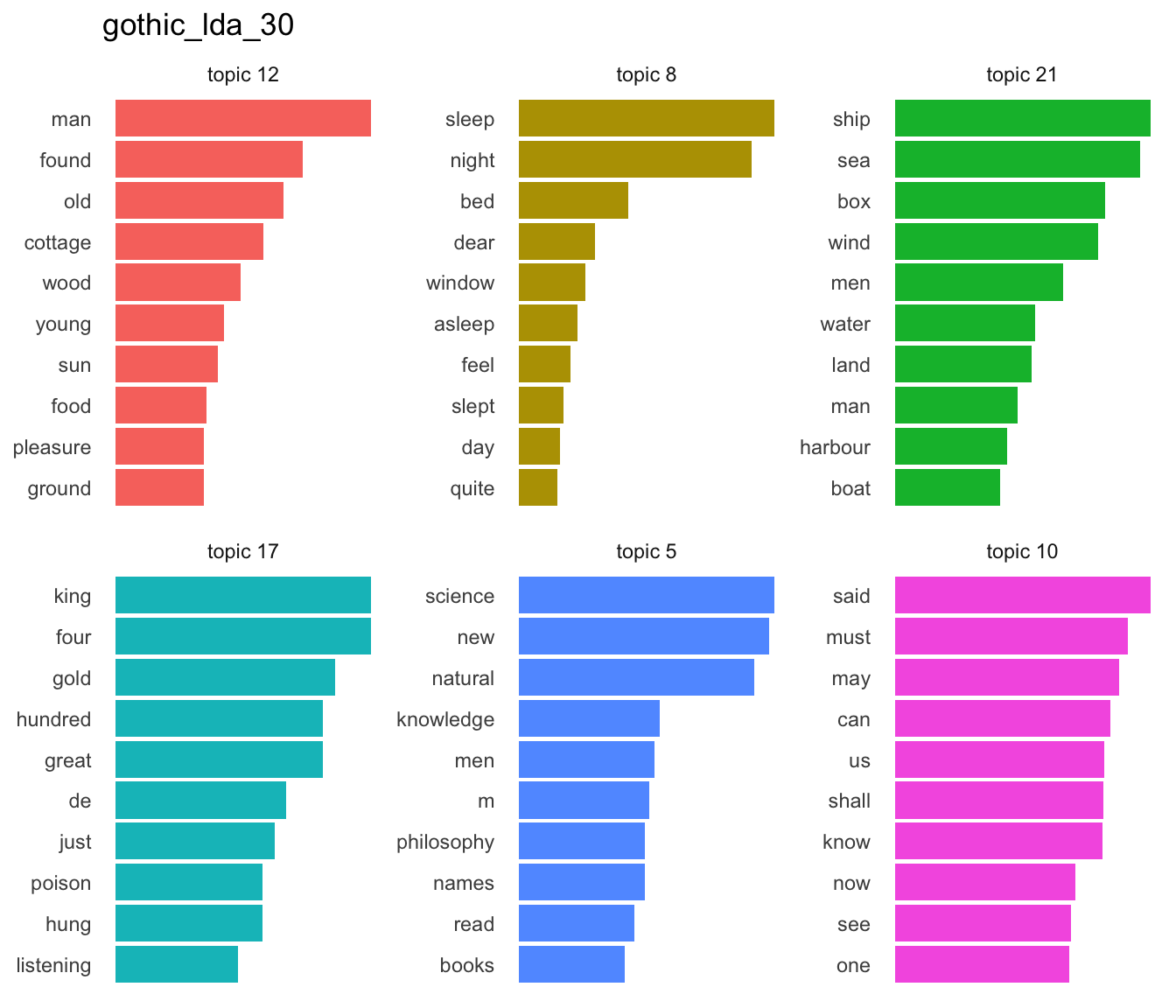
Right away I have a sense for some of these.
Topic 12 is one I recognize from Frankenstein, showing the significant passage in which the creature learns how to be human by watching the family in the cottage.
Topic 21 is clearly about sea travel. This must be an important part of Dracula at a few points in that novel.
Topic 5 shows the part of Frankenstein when Victor Frankenstein was learning all he needed to make his creation.
Topic 10 clearly shows a “junk” topic of common words.
5.3 Topics as word clouds
Bar charts are great for studying the top 5 or 10 words in a topic, but that might not be enough to get a good sense of what the topic is. Diving more deeply into a topic can yield greater insight into it, and word clouds are great for visualizing a larger number of words. The visualize_topic_wordcloud() function makes that possible. Just like the other visualize_...() functions, it also saves images into the “plots” folder. Let’s use it to look more closely at a couple topics considered above. First is topic 12:
visualize_topic_wordcloud(gothic_lda_30, 12)
Seeing these words in context gives a sense of what’s happening in these crucial scenes of Frankenstein. By watching these strangers, the creature learns language, begins to appreciate the love they have for each other, and starts to understand the sadness in his own loneliness. The word cloud makes clear what topic 12 is about, and seeing it in the distribution chart for Frankenstein makes clear how pivotal this topic is to that text.
Now here’s topic 24, which featured in both Frankenstein and The Castle of Otranto:
visualize_topic_wordcloud(gothic_lda_30, 24)
It’s very clear that this topic deals with the idea of trauma, perhaps after the murder of some innocent victim. And these themes are prevalent in both books, with characters reacting to Manfred’s killing by a giant helmet in Otranto and Victor’s dealing with the death of both William and Elizabeth by the creature in Frankenstein. (Oops, spoilers for these multi-hundred-years-old books!)
If it hadn’t been for topic modeling, I might have overlooked shared elements of these texts: In both The Castle of Otranto and Frankenstein, action is driven by the murder of innocent victims; in both, surviving family members seek vengeance, understanding, or release.
6 Exploring interactively
We use visualization to communicate our findings, but we also use it to explore the data. And while we explore, we might wish to move quickly, seeing and learning in one step, instead of taking two steps to see the topic distribution and then discover what a topic is about. For this reason, the function interactive_document_topics() will add interactivity to the topic distributions, letting us mouse around and peek into some of the top words for topics:
interactive_document_topics(gothic_lda_30, top_n = 6)I wish I could make this last version look more like the non-interactive versions, but there are tradeoffs among useful, helpful, and easy!
Footnotes
This step, especially, is inspired by the “‘Secret’ Recipe for Topic Modeling Themes,” by Matthew Jockers.↩︎
Citation
BibTeX citation:
@misc{clawson2023,
  author = {Clawson, James},
  title = {Finding {Topics} in {Text} {Data}},
  date = {2023-08-02},
  url = {https://jmclawson.net/posts/topic-modelling/},
  langid = {en}
}
For attribution, please cite this work as:
Clawson, James. “Finding Topics in Text Data.” jmclawson.net, 2 Aug. 2023, https://jmclawson.net/posts/topic-modelling/.